In this speedy marathon we will learn some basics of Registration Act and Delhi Rent Control Act applicablity in case of Rent Agreement is made for more than 12 Months

Let's understand.

• What is rent Agreement

It is an written agreement between landlord and tenant whereon both agrees on such terms and conditions mentioned therein.

• Is Stamp paper is mandatory for this agreement.

Yes. Normally we use Stamp Paper of value Rs. 50 or Rs. 100 and this can be done by any Notary Public easily.

• Now what will happen if we increase the tenure of lease/rent agreement more than 11 months

First of all we have to understand which documents are required to be register.

Applicablity of Registration Act 1908

As per Section 17 of Registration Act 1908 documents mentioned in Section 17 are mandatorily required to be registered.

As far as if we talk about Rent/lease agreement made for equal to or more than 12 months it will attract Stamp duty as well as registration of document becomes neccessary 

Applicablity of Delhi rent Control Act

If amount of rent charged by landlord is upto 3500 in that case the above act shall become applicable.

However amount charged by landlord is more than Rs. 3500 in that case benefit of Delhi Rent Control Act shall not work in the favour of tenent

What kind of benefit is given under Delhi Rent Control Act.

In case of dispute arised between landlord and tenant in that case tenant has been given some rights against landlord no need to go to any arbitration or court. Otherwise this Act won't  work in favour of tenant.

(1) In every proceeding of the recovery of possession of any premises on the ground specified in clause (a) of the proviso to sub-section (1) of section 14, the Controller shall, after giving the parties an opportunity of being heard, make an order directing the tenant to pay to the landlord or deposit with the Controller within one month of the date of the order, an amount calculated at the rate of rent at which it was last paid for the period for which the arrears of the rent were legally recoverable from the tenant including the period subsequent thereto up to the end of the month previous to that in which payment or deposit is made and to continue to pay or deposit, month by month, by the fifteen of each succeeding month, a sum equivalent to the rent at that rate.

(2) If, in any proceeding for the recovery of possession of any premises on any ground other than that referred to in sub-section (1), the tenant contest the claim for eviction, the landlord may, at any state of the proceeding, make an application to the Controller for an order on the tenant to pay to the landlord the amount of rent legally recoverable from the tenant and the Controller may, after giving the parties an opportunity of being heard, make an order in accordance with the provisions of the said sub-section.

(3) If, in any proceeding referred to in sub-section (1) or sub-section (2), there is any dispute as to the person or persons to whom the rent is payable, the Controller may direct the tenant to deposit with the Controller the amount payable by him under sub-section (1) or sub-section (2), as the case may be until the standard rent in relation thereto is fixed having regard to the provisions of this Act, and the amount of arrears if any, calculated on the basis of the standard rent shall be paid or deposited by the tenant within one month of the date on which the standard rent is fixed or such further time as the Controller may allow in this behalf.

(4) If, in any proceeding referred to in sub-section (1) or sub-section (2), there is any dispute as to the person or persons to whom the rent is payable, the Controller may direct the tenant to deposit with the Controller the amount payable by him under sub-section (1) or sub-section (2) or sub-section (3), as the case may be, and in such a case no person shall be entitled to withdraw the amount in deposit until the Controller decides the dispute and makes an order for payment of the same.

(5) If the Controller is satisfied that any dispute referred to in sub-section (4) has been raised by a tenant for reasons which are false or frivolous, the Controller may order the defense against eviction to be struck out and proceed with the hearing of the application.

(6) If a tenant makes payment or deposit as required by sub-section (1) or sub-section (3), no order shall be made for the recovery of possession on the ground of default in the payment of rent by the tenant, but the Controller may allow such costs as he may deem fit to the landlord.

(7) If a tenant fails to make payment or deposit as required by this section, the Controller may order the defense against eviction to be struck out an proceed with the hearing of the application.

Due to Covid 19 Pandemic, almost all the due dates for filling returns, taxes and required documents to the government has been extended but for the individual whose self assessment tax liability for the Financial Year 2019-20 exceeds Rs. 1 lakh, the last date of submitting income tax liabilities for the same is 31st July, 2020 after that penal interest of 1 per cent per month would be levied on any short payment of this.. The government wants a certain category of tax payers to pay their entire income tax liability for FY 2019-20 even before they get to know their full income and the TDS on it.

Here’s how this anomaly has arisen.

As per the government notification effective June 30,2020, all tax payers with total self assessment tax liability for F.Y. 2019-20 exceeding Rs 1 lakh must pay all of it by July 31, 2020 else penal interest of 1 per cent per month under section 234A of the Income-tax Act would be levied on any short payment of this.

However, the last date for banks and other deductors of tax at source such as employers etc, to file TDS returns and issue TDS certificates for last quarter of FY 2019-20 is July 31 and August 15, 2020, respectively. These two deadlines were advanced from the normal due dates of May 31 and June 15, respectively, due to the Covid 19 pandemic. Individuals whose tax has been deducted at source (e.g. interest paid on cumulative fixed deposits, salary etc.) normally get to know the full amount paid to them (income) and the TDS on it, only when these figures start reflecting in their Form 26AS on the income tax website or when the deductor issues the related TDS certificates to them. However, normally these figures start to show in Form 26AS only after the deductor files it’s TDS return with the income tax department. As the last date by which deductors have to issue TDS certificates for last quarter of F.Y. 2019-20 is August 15, the earliest an individual tax payer can expect to know the income and TDS figures definitively is by July 31 which is the deadline for deductors to file their TDS returns.

The most common types of income on which TDS is deducted, if applicable, include interest on fixed deposits with banks, non-banking finance companies, corporates etc and salary paid by employers. Although it is possible, for an individual to estimate his/her income from these sources, the exact amount paid and the TDS from those payments can only be known once these figures start to show in the Form 26AS of the individual. TDS certificates are normally issued after that.

Although some deductors have filed their TDS returns and are issuing TDS certificates, many others, such as the post office (on Senior citizen saving schemes), may not have done so because as per law they have time till July 31. The deadline to issue TDS certificates is of course even later.

“The result of the above situation is that individuals whose income suffers TDS to a large extent, will face problems in calculating their total income and the tax already deducted on it. Consequently, they will be unable to calculate exact amount of the self assessment tax payable on their total income by July 31. Therefore, paying the correct amount in full by July 31 becomes very difficult. Alternatively, they may end up paying more to avoid penal interest and have to claim a refund,” 

However, clearly the government wants that these individuals should pay the full self assessment tax by July 31 even though they may not be able to know their exact income and TDS by then.

Relative Information about the extended dates of filling returns are as follows: 

(a) The due date to file income tax returns for A.Y. 2020-21 stands extended from 31 July to 30 November 2020. The due date for tax audit stands extended from 30 September 2020 to 31 October 2020. Similarly, the income tax returns filed upon a tax audit are now due by 30 November 2020.

(b) Reduction in TDS and TCS rates by 25% of the present rates, for payments from 14 May till 31 March 2021.

(c) All pending income-tax refunds to be released to non-corporate entities immediately.

(d) The last date for completion of assessments which are getting time-barred on 30 September 2020 stands extended to 31 December 2020. In the case of assessments which get time-barred on 31 March 2021, the time stands extended to 30 September 2021.

(e) The last date of making payment under Vivaad se Vishwas Scheme without additional amount stands extended to 31 December 2020.

Introduction of Excel

Microsoft Excel is a spreadsheet application invented and developed by Microsoft Corporation.

Spreadsheet of Excel is a combination of Columns and Rows. Here column shall be show in alphabetic order like A, B, C ………so on and row is in numeric order like 1, 2, 3, …………….. so on.

Total column and Total Row

Column 16,384 (Name of last column is XFD)

Row 10,48,576

How to launch Excel

1. Click on the Start Button.

2. In the Search Program and Files box type Excel.

3. Click on Excel 2013 from the Program results.

4. The Microsoft Excel 2013 program will open

OR

1. Press the Windows key on the keyboard.

2. Type Excel.

3. Click on Excel 2013 under the Apps results.

OR

1.. Press Window key and R(Run)

2. Type excel in dialogue box

3. Press Enter

Excel Overview

The Excel Interface given in the image given below:

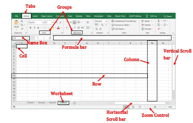
Understanding of cells

if you all see in Spreadsheet thousands of rectangles are there to see and these rectangles are occurring of intersection of column and row. Those rectangles are called as cells. Every cell has own name and name should be based on column and row.

Cell

Every cell has its own name, or cell address, in light of its segment and line. In this model, the chose cell crosses segment C and column 5, so the cell address is C5. The cell address will likewise show up in the Name box. Note that a cell's segment and line headings are featured when the cell is chosen.

Mouse Cursors are available in excel for different purposes.

The Five most important shapes are as follows:

 

	Using for Selection a cell or more than one cells.
	The Auto fill handle. Used for copying formula or extending a data series.
	To select cells on the worksheet. Selects whole row/column when positioned on the number/letter heading label.
	At borders of column headings. Drag to widen a column.
	At borders of row letters. Drag to increase height of row.

Excel Home Tab 

The Excel Home Tab is utilized to perform regular orders, for example, Bold, underline, Copy, and Paste. It is additionally used to apply formatting to cells in a worksheet.

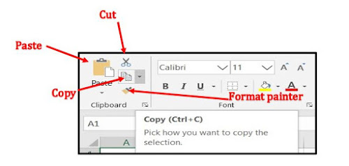
Clipboard Group

1.    Paste: To insert data that has been placed on the clipboard into a worksheet cell, click this button.

 

2.    Cut: This button is used to remove data from a worksheet cell and place it on the clipboard. Once the data has been placed on the clipboard, it can be inserted into another cell in the same worksheet or into a different worksheet.

 

3.    Copy : To copy data from a cell in a worksheet so that it can be placed into another area of the worksheet, click this button. The data that is copied is placed on the clipboard.

 

4.    Format Painter: Click this button to apply formatting from one cell in a worksheet to another cell or range of cells in the same worksheet. Clicking the button once will apply the formatting to only one other cell or range. Double-clicking makes it possible to apply the formatting to more than one cell or range of cells.

Font Group

Font Type: This button is used to change the style of the font within a cell or a range of cells in a worksheet. A list of different font styles will appear. Move the mouse pointer over the style to see a Live Preview.

 

Font Size: To change the size of the font in a cell or range of cells in a worksheet, click this button. Move the mouse pointer over each of the sizes to see a Live Preview. A list of different font sizes will

appear. Click the desired size to select it.

Increase Font Size: This button is used to increase the font size within a cell or range of cells. Each time the button is clicked, the size of the font increases by one or two points.

Decrease Font Size: Click this button to decrease the size of the font by one or two point increments. Each time the button is clicked, the size of the font will decrease one or two points.

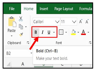
To use the Bold, Italic, and Underline commands

 1. Select the cell(s) you wish to modify.

2. Click the Bold (B), Italic (I), or Underline (U) command on the Home tab. In our example, we'll make the selected cells bold.

3. The selected style will be applied to the text.

  

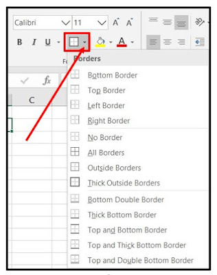
Border Style

Allow you to create clear and defined boundaries for different sections of your worksheet.

To add a border

1. Select the cell(s) you wish to modify.

2. Click the drop-down arrow next to the Borders command on the Home tab. The Borders drop-down menu will appear.

 3. Select the border style you want to use.

4. The selected border style will appear.

Cell borders and fill colors

TIP: You can draw borders and change the line style and color of borders with the Draw Borders tools at the bottom of the Borders drop-down menu 

1.   To add a fill color 

1. Select the cell(s) you wish to modify. 

2. Click the drop-down arrow next to the Fill Color command on the        Home tab. The Fill Color menu will appear.

3. Select the fill color you want to use. A live preview of the new fill color will appear as you hover the mouse over different options. In our example, we'll choose Light Green.

4.  The selected fill color will appear in the selected cells.

To change the font color 

1. Select the cell(s) you wish to modify.

2. lick the drop-down arrow next to the Font Color command on the Home tab. The Color menu will appear.

3. Select the desired font color. A live preview of the new font color will appear as you hover the mouse over different options. 

4.    The text will change to the selected font color. 

Text Alignment Group 

By default, any text entered into your worksheet will be aligned to the bottom-left of a cell. Any numbers will be aligned to the bottom-right of a cell. Changing the alignment of your cell content allows you to choose how the content is displayed in any cell, which can make your cell content easier to read.

To change horizontal text alignment

1. Select the cell(s) you wish to modify.

2. Select one of the three horizontal alignment commands on the Home tab. In our example, we'll choose Center Align.

3. The text will realign.

To change vertical text alignment 

1. Select the cell(s) you wish to modify.

2. Select one of the three vertical alignment commands on the Home tab. In our example, we'll

choose Middle Align.

3. The text will realign. 

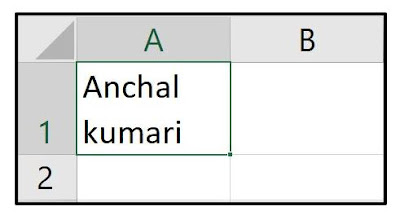
Wrap Text

Wrap text by Excel in the event that you need to show long content on various lines in a current cell. Wrap text naturally or enter a manual line break.

Ø Take an example, Type a long text in cell A1 

 

Ø Select Cell A1 and go to Home Tab>>Alignment Group>> click on Wrap Text

 

Ø Result: 

Merge and Center

This option merge selected cells into one cell.

Ø Let’s take an example 

There is marksheet below and we need a heading above of data with 

full range of marksheet. 

see as screen given below: 

 

 

Ø Select Cell A1 and go to Home Tab>>Alignment Group>> click on Merge & Center.

 

 

Ø Result:

 

 

 

 Style Group

Conditional formatting

Conditional formatting permits you to consequently apply arranging, for example, Colors, Icon and Data bars—to at least one cells dependent on the cell esteem. To do this, you'll have to make a Conditional formatting rule.

For Example: if we want to the highlight the value more than 30,000 in Total column of salary sheet.

Step 1: Select the range you want to apply the rule.

Step 2:

Click to Conditional formatting option >> Highlight Cell Rules>> Greater than

Step 3: put the value in dialogue box and see the RESULT:

Let’s take another example: we want to highlight more than 18,000 in all salary sheet data.

Follow same step as earlier example:

1. Select data from Basic to HRA column.

2. Follow same step to conditional formatting and highlight greater than rule:

In Conditional Formatting several option to represent data in another format

·      Data Bar: Data bar like horizontal bar in each cell and rule apply according to cell value in descending order/largest to smallest value.

See the image given below:

STEP: Click to Conditional formatting

option >> Data bar

 

 

       

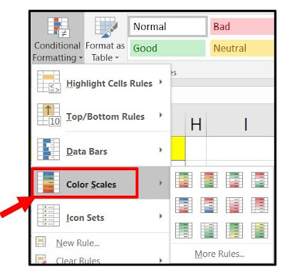
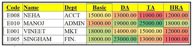
 Color Scale: Color Scales change the color of each cell based on its

value. Each color scale uses a two- or three-color gradient. For

example, in the Green-Yellow-Red color scale, the highest values are 

green,the average values are yellow, and the lowest values are red.

STEP: Click to Conditional formatting option >> Color scale

·      Icon Set: Specific or dynamic icon set on based on cell value.

STEP: Click to Conditional formatting option >> Icon Set

If we want to remove any conditional formatting so follow the step given below:

Select the area and Go To Conditional Formatting >> Clear Rules >> Clear Rules from Selective Cells/ Clear Rules from Entire Sheet.

Format as Table

When you've entered data into a worksheet, you might need to organize your information as a table. Much the same as ordinary arranging, tables can improve the look and feel of your exercise manual, yet they'll likewise assist with sorting out your substance and make your information simpler to utilize. Exceed expectations incorporates a few instruments and predefined table styles, permitting you to make tables rapidly and without any problem.

Let’s go and see a normal data apply with format as table with the help of picture:

Step 1: we have to select all data or put the mouse cursor in the any one cell of data.

Step 2: Go to Format as Table>> select any style as per the choice.

RESULT:

Cell styles

Rather than formatting cells manually, you can use Excel's predesigned cell styles. Cell styles are a quick way to include professional formatting for different parts of your workbook, such as titles and headers.

To apply a cell style

1. Select the cell(s) you wish to modify.

2. Click the Cell Styles command on the Home tab, then choose the desired style from the drop-down menu.

3. The selected cell style will appear.

Cell Group

In this article, I am demonstrating how to Insert-Delete-Format cells in Excel worksheets. Presently through to home tab in Excel worksheets, you have a Group of orders which named Cell. The cell Group contains a few orders and alternatives which are discussing the cell. Inside every cell, we can do a ton of figuring, and every phone is significant for our assignment. Presently there are three choices which are the most significant, presently I will give you some data about these three choices the show the uses.

 

Insert: Here you can become known about inserting a cell, sheet rows, sheet columns, and Insert another sheet.

Delete: if you have any useless cell, rows, columns, and worksheet you can delete it easily

Format: Cell design contains a few choices which can assist you with changing the size of your cells. Hide and Unhide the cells, arrange sheets, and Protection.

Cell Size: – In this option we can change the height of rows and width of the columns, and also you can set a Autofit Row Height.

Visibility: – Here you can hide and unhide your cells, rows, columns, and sheets.

Organize Sheets: – Now you can rename the sheet as per your need and move or copy your sheet. And if you want to change tab color, so you can change too.

         

Editing Group

Auto sum: On the off chance that you have to sum a row or column of numbers, let Excel figure it out for you. Select a cell close to the numbers you need to total, click AutoSum on the Home tab, press Enter, and you're finished. Shortcut keys of AutoSum is (“Alt”+”=”).

Fill: You can use the Fill command to fill a formula into a Selective range of cells. You can do the following:

1.    Select the cell with the formula and the range of cells you want to fill.

2.    Click Home > Fill, and choose either Down, Right, Up, or Left as per your need of direction.
shortcut keys:

a.    Down Drag: Ctrl+D

b.    Right Drag: Ctrl+R

Series: The Excel Fill Series tool is like having a bundle of usage. It can help with one of the most common tasks we do in Excel, which is to create a serial numbers like 1,2,3,….. so on and 1,3,5,…… so on and also date fill. Fill Series option can easily handle them all.

for an example: create a series from 1 to 20 put 1 into any of cell and select that cell

Go to > home tab> editing group>fill> series

Follow the step as given image.

Result:

If u want to fill series in odd and even number series you have to set step value as per your need.

Like if you want to odd number like 1,3,5…………..

So, you have to write 1 in any cell and select of it and follow same step as above but you have to taken step value 2 for odd number and as same for even number series.

 

Clear:

 If you want clear all data or clear formatting of data and some others also available of clear option.

Go to > home tab>editing group> clear

Sort & filter:

Sort: if you want to sort your data in A to Z or vice versa and Numbers data in smallest to largest or vice versa

So, you can use sort option for that.

Go to>home tab>editing group> Sort & filter

You can see in image of option of A to Z and Z to A.

If you want to select option from Smallest to Largest or vice versa you can select the range of numbers data. It will be shown as smallest to largest or vice versa automatically.

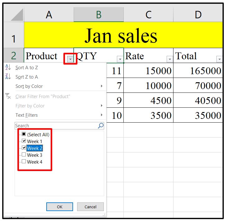
Filter: you can easily filter your large number of data in very easy option that

is filter

Go to > home tab>editing group> Sort & filter

Let’s see usage of this option with an example:

We have some number of data given below:

Click on filter button and click on product filter button:

Result:

Find & Select:

Find: When working with a large number of data in Excel, it can be difficult and time consuming to locate specific information. You can easily search using the Find feature.

Go to > home tab > editing group> Find & Select

Let’s take an example:

Click on find option and type manoj to find.

Result:

Cursor of mouse Automatically go to cell where Manoj name available.

Replace

Let’s take a same example as above for replace options:

Click on Replace option and type Manoj in find and type Saroj in replace option.

Go To:

If you want to go any specific cells in entire worksheet

Use go to option for that

Go to > Home Tab > Editing > go to

Step 1

Click on go to and type cell name where you want to go.

 

Result: